Motion in dipole magnetic field#

This notebook demonstrates a basic GT simulation workflow for numerically integrating the equation of motion of a charged particle in the Earth’s magnetic field approximated by a dipole model.

Goals of this example:

Define the Dipole magnetic field and initial conditions for a single particle (a 10 MeV proton).
Compute the trajectory with two integrators: Buneman–Boris (BB) and 6th‑order Runge–Kutta (RK6).
Visually compare trajectories in the XY plane and estimate a characteristic cyclotron motion scale (the Larmor radius) along the trajectory.

Expected output:

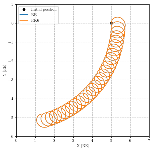
A plot of BB and RK6 trajectories starting from the same point and showing the difference in the results of calculations using two numerical schemes for a selected time step.
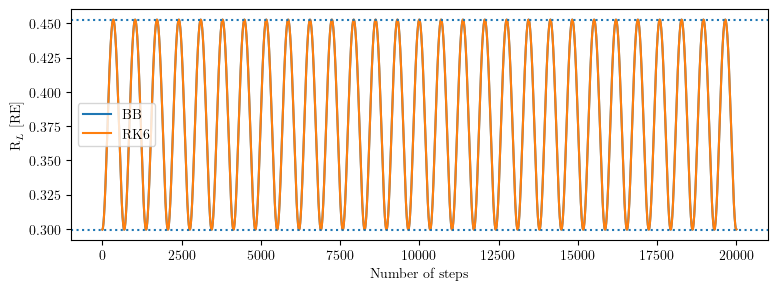
A plot of the Larmor radius versus step index (for both methods), including the minimum/maximum (R_L) over the simulated interval.

from datetime import datetime

import matplotlib.pyplot as plt
import numpy as np
from gtsimulation.pusher import BunemanBorisSimulator, RungeKutta6Simulator
from gtsimulation.common import Regions, Units
from gtsimulation.magnetic_field.magnetosphere import Dipole
from gtsimulation.particle import generator, Flux

Problem setup: field, particle, and integration parameters#

This section defines the simulation setup:

date (used by time-dependent field models);
the Magnetosphere region and the Dipole field model;
particle initial conditions: a single 10 MeV proton starting at ([5 R_E, 0, 0]) point in the geocentric coordinate system (also known as ECEF) with an initial velocity directed along (Y) axis;
integration settings: total simulated time total_time, number of steps n_steps, and time step dt;
which quantities to store in the track (coordinates, velocities, energy, and magnetic field values along the trajectory).

The expected outcome of this block is a fully defined configuration that can be passed to different numerical schemes for comparison.

date = datetime(2008, 1, 1)
region = Regions.Magnetosphere
b_field = Dipole(date=date)
medium = None

particle = Flux(
    Spectrum=generator.spectrum.Monolines(energy=10 * Units.MeV),
    Distribution=generator.distribution.UserInput(
        R0=np.array([5 * Units.RE, 0, 0]),
        V0=[0, 1, 0]
    ),
    Names="proton",
    Nevents=1
)

use_decay = False
nuclear_interaction = None

total_time = 10  # total time [s]
n_steps = 20000
dt = total_time / n_steps
break_conditions = None

save = [1, {"Coordinates": True, "Velocities": True, "Energy": True, "Bfield": True}]
output = None

verbose = 0

Trajectory computation: Buneman–Boris (BB) scheme#

This block creates a BunemanBorisSimulator instance and runs the particle trajectory calculation in the given magnetic field.

After execution, the following arrays are extracted:

r_BB — trajectory coordinates,
v_BB — velocities,
T_BB — particle energy along the trajectory,
B_BB — magnetic field sampled at trajectory points.

The output arrays of coordinate, velocity and field vectors are also expressed in the geocentric coordinate system.

The expected result is a stable trajectory (BB is a common choice for particle tracing in electromagnetic fields) and a dataset suitable for comparison with other integrators.

simulator_BB = BunemanBorisSimulator(
    Bfield=b_field,
    Region=region,
    Medium=medium,
    Particles=particle,
    InteractNUC=nuclear_interaction,
    UseDecay=use_decay,
    Date=date,
    Step=dt,
    Num=n_steps,
    BreakCondition=break_conditions,
    Save=save,
    Output=output,
    Verbose=verbose
)

track_BB = simulator_BB()[0][0]
r_BB = track_BB["Track"]["Coordinates"]
v_BB = track_BB["Track"]["Velocities"]
T_BB = track_BB["Track"]["Energy"]
B_BB = track_BB["Track"]["Bfield"]

Trajectory computation: 6th-order Runge–Kutta (RK6)#

This block repeats the same calculation for the same initial conditions, but using the RungeKutta6Simulator integrator.

After execution, the arrays

r_RK6, v_RK6, T_RK6, B_RK6 are obtained analogously to the BB case.

The expected result is that the RK6 trajectory closely matches the BB trajectory for a sufficiently small dt, with possible small differences due to method properties and numerical error accumulation.

simulator_RK6 = RungeKutta6Simulator(
    Bfield=b_field,
    Region=region,
    Medium=medium,
    Particles=particle,
    InteractNUC=nuclear_interaction,
    UseDecay=use_decay,
    Date=date,
    Step=dt,
    Num=n_steps,
    BreakCondition=break_conditions,
    Save=save,
    Output=output,
    Verbose=verbose
)

track_RK6 = simulator_RK6()[0][0]
r_RK6 = track_RK6["Track"]["Coordinates"]
v_RK6 = track_RK6["Track"]["Velocities"]
T_RK6 = track_RK6["Track"]["Energy"]
B_RK6 = track_RK6["Track"]["Bfield"]

Trajectory comparison (BB vs RK6)#

This section plots the trajectories in the XY plane (in Earth radii (R_E)):

the starting point is marked explicitly;
trajectories computed with BB and RK6 are overlaid.

The expected output is a clear visual comparison of the trajectories calculated using the two numerical schemes. At the chosen time step dt, discrepancies in the trajectories become visible, and these discrepancies accumulate.

fig = plt.figure(figsize=(6, 6))
ax = fig.subplots()

ax.scatter(5, 0, label="Initial position", color="black")
ax.plot(*r_BB.T[:2] / Units.RE, label="BB")
ax.plot(*r_RK6.T[:2] / Units.RE, label="RK6")

ax.set_xlim(0, 7)
ax.set_ylim(-6, 1)
ax.set_xlabel("X [RE]")
ax.set_ylabel("Y [RE]")
ax.set_aspect("equal")
ax.grid(True, linestyle="--", alpha=0.8)
ax.legend()

plt.show()

../../_images/2fb0941ad032a0cd9969d355d008ef4bf7218b0226da18dd6545c392859b81d1.png

Estimating the Larmor radius along the trajectory#

This section evaluates a characteristic spatial scale of the cyclotron motion—the Larmor radius (R_L)—as a function of time/step index.

Workflow:

import GetLarmorRadius;
read particle mass and charge from the simulation output;
compute the pitch angle (angle between velocity and magnetic-field direction) and then (R_L) at each trajectory point;
plot (R_L) (in (R_E)) for BB and RK6 and indicate the minimum/maximum values.

The expected output is two close (R_L) curves and an understanding of how the local Larmor radius changes as the particle moves through a non-uniform dipole field.

from gtsimulation.magnetic_field.magnetosphere.Additions import GetLarmorRadius

M = track_BB["Particle"]["M"]
Z = track_BB["Particle"]["Ze"]

B_unit_BB = B_BB / np.linalg.norm(B_BB, axis=1)[:, None]
v_dot_B_BB = np.sum(v_BB * B_unit_BB, axis=1)
pitch_BB = np.rad2deg(np.arccos(v_dot_B_BB))  # clearly get a pitch angle of 90 degrees
LR_BB = GetLarmorRadius(T_BB, np.linalg.norm(B_BB, axis=1), Z, M * Units.MeV2kg, pitch_BB)

B_unit_RK6 = B_RK6 / np.linalg.norm(B_RK6, axis=1)[:, None]
v_dot_B_RK6 = np.sum(v_RK6 * B_unit_RK6, axis=1)
pitch_RK6 = np.rad2deg(np.arccos(v_dot_B_RK6))  # clearly get a pitch angle of 90 degrees
LR_RK6 = GetLarmorRadius(T_RK6, np.linalg.norm(B_RK6, axis=1), Z, M * Units.MeV2kg, pitch_RK6)

fig = plt.figure(figsize=(9, 3))
ax = fig.subplots()

ax.plot(LR_BB / Units.RE, label="BB")
ax.plot(LR_RK6 / Units.RE, label="RK6")

ax.axhline(y=np.min(LR_BB / Units.RE), linestyle=":")
ax.axhline(y=np.max(LR_BB / Units.RE), linestyle=":")

ax.set_xlabel("Number of steps")
ax.set_ylabel("R$_L$ [RE]")
ax.legend(loc="center left")

plt.show()

../../_images/795baf4c127e41b186877e6bf6f3a1f57debf1f697dba909528f0632bd0aef39.png