Deflection in Galaxy

This notebook demonstrates the simulation of Ultra-High-Energy Cosmic Ray (UHECR) propagation through the Galaxy. The goal is to estimate the deflection of protons with energies \(E = 60~\text{EeV}\) caused by the Galactic magnetic field (GMF).

At such high energies (\(> 10^{18}\) eV), the Larmor radius of particles becomes comparable to the size of the Galaxy, and diffusion effects are negligible. Therefore, we can simulate their propagation using trajectory backtracing:

• Launch antiparticles (antiprotons) from the Solar System in various directions covering the celestial sphere.

• Trace them through the GMF model (Jansson & Farrar, JF12) until they escape the Galactic halo.

• Calculate the angle between the initial launch direction and the final position vector.

The deflection angle \(\alpha\) is calculated as:

\[ \alpha = \arccos\left( \frac{\mathbf{v}_0 \cdot (\mathbf{r}_f - \mathbf{r}_0)}{|\mathbf{r}_f - \mathbf{r}_0|}\right) \]

where:

• \(\mathbf{v}_0\) is the initial normalized velocity vector (direction of observation),

• \(\mathbf{r}_0\) is the starting position (Solar System),

• \(\mathbf{r}_f\) is the final position where the particle escapes the Galaxy.

Expected Output:

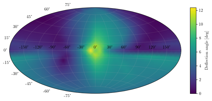
A sky map (Galactic coordinates) showing the magnitude of deflection for 60 EeV protons, highlighting the anisotropic influence of the large-scale magnetic field structure.

from datetime import datetime

import matplotlib.pyplot as plt
import numpy as np
from gtsimulation.pusher import BunemanBorisSimulator
from gtsimulation.common import Regions, Units
from gtsimulation.magnetic_field.galaxy import JF12mod
from gtsimulation.particle import generator, Flux

Simulation settings

We define the global simulation environment:

• Magnetic Field: Jansson & Farrar (2012) model (JF12), random component disabled (use_noise=False) to study the regular field effect.

• Region: Galaxy.

• Time Step: Large step (\(1000\) days) is sufficient for UHECRs due to their immense rigidity.

• Break Conditions: Simulation stops when the particle reaches the Galactic halo boundary (\(R > 28.5\) kpc).

date = datetime(2025, 1, 1)
region = Regions.Galaxy
b_field = JF12mod(use_noise=False)
medium = None

use_decay = False
nuclear_interaction = None

dt = 1000 * Units.day  # time step [s]
n_steps = int(1e5)

# dt = 100 * Units.day  # time step [s]
# n_steps = int(1e6)

break_conditions = [{"Rmax": 28.5 * Units.kpc}, np.array([-8.5, 0, 0]) * Units.kpc]

save = [0, {"Coordinates": True, "Velocities": True}]
output = None

verbose = 0

The function get_deflection_angle performs the core logic for a single direction \((l, b)\):

• Converts Galactic coordinates \((l, b)\) to a velocity vector.

• Initializes an anti-proton at the Solar System location \((-8.5, 0, 0)\) kpc.

• Runs the BunemanBorisSimulator.

• Computes the deflection angle \(\alpha\) using the formula defined in the introduction.

def get_deflection_angle(l, b):
    v = np.array([
        np.cos(np.deg2rad(l)) * np.cos(np.deg2rad(b)),
        np.sin(np.deg2rad(l)) * np.cos(np.deg2rad(b)),
        np.sin(np.deg2rad(b))
    ])
    particle = Flux(
        Spectrum=generator.spectrum.UserInput(energy=60 * Units.EeV),
        Distribution=generator.distribution.UserInput(
            R0=np.array([-8.5, 0, 0]) * Units.kpc,
            V0=v
        ),
        Names="anti_proton"
    )
    simulator = BunemanBorisSimulator(
        Bfield=b_field,
        Region=region,
        Medium=medium,
        Particles=particle,
        InteractNUC=nuclear_interaction,
        UseDecay=use_decay,
        Date=date,
        Step=dt,
        Num=n_steps,
        BreakCondition=break_conditions,
        Save=save,
        Output=output,
        Verbose=verbose
    )
    event = simulator()[0][0]
    r_0 = event['Particle']['R0']
    r_f = event['Track']['Coordinates'][-1]
    v_0 = event['Particle']['V0']
    angle = np.acos(np.dot(v_0, (r_f - r_0)) / np.linalg.norm(r_f - r_0))
    return np.rad2deg(angle)

Global scan setup

We define a grid in Galactic coordinates \((l, b)\) to map the deflection angles across the entire sky.

• Longitude \(l\): -180 to 180 degrees.

• Latitude \(b\): -90 to 90 degrees.

from joblib import Parallel, delayed
from tqdm_joblib import tqdm_joblib

from mpl_toolkits.axes_grid1 import make_axes_locatable

/home/rustam/Documents/Work/MEPhI/software/GTsimulation/.venv/lib/python3.12/site-packages/tqdm_joblib/__init__.py:4: TqdmExperimentalWarning: Using `tqdm.autonotebook.tqdm` in notebook mode. Use `tqdm.tqdm` instead to force console mode (e.g. in jupyter console)
  from tqdm.autonotebook import tqdm

l_grid = np.arange(-180, 180, 10)
b_grid = np.arange(-90, 91, 10)
a_grid = np.empty((b_grid.size, l_grid.size))

Since each direction is independent, we use joblib to parallelize the computation across all available CPU cores.

def worker(i_l, i_b):
    angle = get_deflection_angle(l_grid[i_l], b_grid[i_b])
    return i_l, i_b, angle

tasks = [(i, j) for i in range(l_grid.size) for j in range(b_grid.size)]
with tqdm_joblib(total=len(tasks)):
    res = Parallel(n_jobs=-1)(delayed(worker)(i, j) for i, j in tasks)
for i_l, i_b, v in res:
    a_grid[i_b, i_l] = v

# add the 180° meridian and copy values from the -180° meridian in order to stitch the map seamlessly
l_grid = np.hstack((l_grid, 180))
a_grid = np.pad(a_grid, pad_width=((0, 0), (0, 1)), mode="wrap")

Visualization

We present the results in two formats:

• Rectangular Projection: Useful for inspecting the raw data grid.

• Mollweide/Aitoff Projection: Standard astronomical projection for full-sky maps.

fig = plt.figure(figsize=(8, 4))
ax = fig.subplots()

pcm = ax.pcolormesh(l_grid, b_grid, a_grid, vmin=0)
ax.set_xlim(-180, 180)
ax.set_ylim(-90, 90)

ax.set_xticks(np.arange(-180, 181, 60))
ax.set_yticks(np.arange(-90, 91, 30))
ax.set_xlabel('Galactic longitude [deg]')
ax.set_ylabel('Galactic latitude [deg]')

divider = make_axes_locatable(ax)
cax = divider.append_axes("right", size="3.5%", pad=0.3, axes_class=plt.Axes)
fig.colorbar(pcm, cax=cax, label="Deflection angle [deg]")

plt.show()

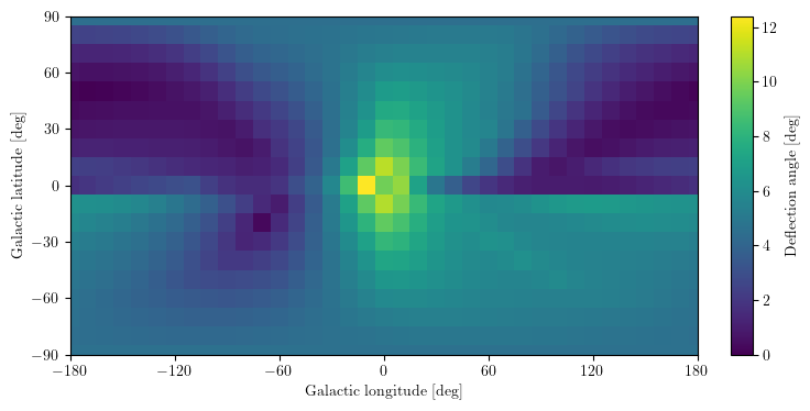
fig = plt.figure(figsize=(8, 4))
ax = fig.add_subplot(111, projection="aitoff")

pcm = ax.pcolormesh(np.deg2rad(l_grid), np.deg2rad(b_grid), a_grid, shading="gouraud", vmin=0)
ax.grid(True, linestyle=':', alpha=0.5)

divider = make_axes_locatable(ax)
cax = divider.append_axes("right", size="3.5%", pad=0.3, axes_class=plt.Axes)
fig.colorbar(pcm, cax=cax, label="Deflection angle [deg]")

plt.show()

# fig.savefig("deflection_angles.pdf")

The resulting map shows the anisotropic nature of UHECR deflection.

• Galactic Plane (\(b \approx 0\)): Higher deflection angles are typically observed due to the stronger magnetic fields in the Galactic disk.

• High Latitudes: Deflections are generally smaller.

Potential ways to improve accuracy:

• Decrease the integration time step (e.g., down to 1 day).

• Increase the latitude/longitude grid resolution.